Numerical Methods for
Inductance Calculation

Part 3 – Solvers, Optimizers, and Empirical Methods

B) Empirical Formulae

Wheeler's Continuous Inductance Formula

In the previous example, we used the Solver routine to find the answer to one specific problem. Each time we change the problem specifications, we need to re-run the solver. This next example demonstrates how to use the solver to develop and to optimize an inductance formula which will then stand on its own, without further need for the solver.

In this example, we refer to this particular inductance formula of Harold Wheeler as "continuous" because he published an earlier formula which is accurate only for long coils which have a length to diameter ℓ/d ratio greater than 0.4. The earlier formula was published in 1928 [16], and is handy if the only means for calculation at your disposal, are a pencil and paper. The fact that you are reading this on a computer screen indicates that there are much more powerful tools now available. The long coil formula was indeed very simple, and for all its simplicity, very accurate within the range of coil geometries for which Wheeler intended it. Unfortunately, virtually every inductance calculator you're likely to find online uses this formula, despite the fact that there are far more accurate formulae available. This in itself is not necessarily a bad thing. The real problem is that many of these calculators come with no warning about the ℓ/d limitation. Even worse, this point where the formula starts to lose accuracy is right in the range where many radio experimenters need to wind their coils. Even more disturbing is the misinformation dispensed on some sites, that this Wheeler formula is the only inductance formula available. Even when Wheeler published his formula, there were far more accurate formulae available. In fact most of the the very accurate formulae that we still use today, were developed prior to 1910, 18 years before Wheeler published his long coil formula. For that reason, and to discourage its further misuse, I won't bother to show Wheeler's long coil formula here at all, though you won't have any problem finding it on the Internet if you really want to search for it. On the other hand, with no searching at all, you can find a superior formula in the next paragraph.

Perhaps as an act of penance, and to encourage people to set aside their crude stone tools, Wheeler published his continuous inductance formula in 1982 [17], 54 years after he published his long coil formula. Reformatted (for consistency with this site), it is:

(30)

where L_S is in µH; d = coil diameter (cm); ℓ = coil length (cm); N = number of turns.

Maximum error is no more than 0.1% for this formula, which is very good considering its simplicity. Note the subscript S on the inductance L_S, which indicates that this is a current sheet formula, and will require round wire corrections for best accuracy.

The purpose of Wheeler's 1982 paper was to demonstrate how one could construct an empirical formula by combining existing analytical formulae. The result is a doubly asymptotic formula, i.e., one that is accurate for both large and small input variables; in this case: both short and long coils.

To begin our analysis, let us recall Nagaoka's formula (3) which is reproduced here:

(3)

By combining (30) and (3) (and correcting for units) we can convert Wheeler's formula into an approximation for Nagaoka's coefficient:

(31)

This is useful, because we have already demonstrated that we can calculate Nagaoka's coefficient to any desired precision (see Part 1a), and so we have a standard against which we can compare Wheeler's formula. A further advantage is that this formula is now a function of a single variable: the shape factor u = d/ℓ.

The following graph shows the relative error in Wheeler's formula by comparing it with a precise calculation of Nagaoka's coefficient.

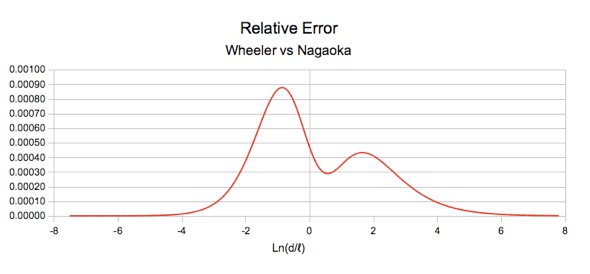
This graph has a logarithmic x-axis, which accentuates the region of interest. As can be seen, the error is all positive, which implies that with some adjustment of coefficients, it may be possible to shift the error down so that the peaks extend equally on either side of zero, with a net reduction in the peak absolute error to half of its previous value.

Wheeler's continuous formula was first made known to me by Rodger Rosenbaum [18] who analysed and modified it, reducing the maximum error to about 0.02%, by adjusting the constants in the denominator of the right side of the formula. His version is as follows:

(32)

As mentioned above, for both very long coils and very short coils, Wheeler's formula (30) converges with the exact current sheet formula. Rodger's version sacrifices the convergence with the exact formula at the extremes while gaining accuracy in the most useful region.

David Knight also analysed the formula [15b], but preserved the asymptotic behaviour for short and long coils by adjusting only zero order constant of 3.2 to 3.244, and the second order constant 1.7636 to 1.7793 resulting in the following:

(33)

This gives a maximum error of 0.0265%  or 265 ppM (parts per million).

At this point, I felt the need to take a crack at it as well, and having the Nelder-Mead solver available, I could let it do all of the hard work. In fact, it was right after I had written the solver code that I needed some examples with which to test it. This formula seemed like a good candidate for study.

Referring back to formula (31), let's look at the fraction on the right, inside the brackets:

When the coil is very short, u becomes very large and the fraction converges towards:

Wheeler explains that 2.3004 is a four decimal place approximation to the exact value:

When the coil is long and u becomes small, the most significant part is 1.7636/u², because of the power of 2. The other two terms become insignificant, and the fraction converges towards:

The value 1.7636 is a four decimal place approximation to the exact value:

These are the two terms that determine the asymptotic behaviour of this inverted polynomial term. However, when combined with the rest of the function, only the 2.3004 value affects the asymptotes of the overall formula. I had, at first, assumed that the second order term, 1.7636, would affect the asymptote of the overall formula at small values of u. As I wanted to maintain correct asymptotic behaviour, I kept the coefficient at its original analytical value for my initial experiments. However, I soon realized that this term does not affect the asymptotes, and therefore, and it is fair game when optimizing the formula.

The 3.2/u term affects the mid-region behaviour, and is purely empirical. This is the bumpy part in the middle of the error graph that we want to flatten.

If asymptotic behaviour is to be preserved, then there is no further optimization possible for the existing terms of the formula beyond what was done by David Knight. However, Rodger Rosenbaum's non-asymptotic version can be further optimized, to 163 ppM (parts per million), by further adjustments of the coefficients. If we want to get more accuracy than that, additional terms must be added, or the entire formula must be changed. To further reduce the error in the mid-region, I considered the possibility of adding another term in the denominator. In order to remain asymptotically correct, the term would have to be greater than degree zero. And there is little benefit in using terms higher than the existing second order term. Possible candidates are a square root term, or more generally, a fractional power term with the exponent between 0 and 2, or a logarithm term; or a combination of these. I tried several combinations of these but eventually found that a single fractional power term gave the best results.

The Wheeler formula optimization is illustrated in the example spreadsheet on the second worksheet entitled 'Wheeler'.

To optimize this formula using a spreadsheet and the solver, we set up a candidate formula (displayed in row 14) with all of the coefficients we wish to adjust grouped together (cell range B5:B10). The candidate formula that was tested is as follows:

Note that the fractional power term has three parameters associated with it: scale factor k4, offset s4 and exponent e4.

Next, we need to come up with an error function. In the tapped coil example given in part 3a, the total error was composed of two parts because there were two specific targets that we wanted to reach: upper and lower frequency. In this case we want to achieve minimum error across the whole range of the function. The approach will be to duplicate the formula on multiple rows in the spreadsheet, and calculate the function for a range of different values of u. On each row we will also calculate Nagaoka's coefficient, then take the difference between the two. Squaring the difference and then summing the result for all of the rows will give us the total error function.

Brief mention was made earlier of the use of the square of the error. It should be mentioned that by summing the squares of each difference value, we are getting a number proportional to the area under the error curve, and so the solver will attempt to minimize this. However that is not our real goal. We want to end up with an empirical function whose worst case error is minimized. We can do this by using spreadsheet max() and min() functions to find the maximum absolute difference (i.e., the value in cell B12) and minimize it. Unfortunately this is not a smooth function, and while it can work, it's often not the best choice, especially if the starting values of input parameters are a long way from the optimum values. The Nelder-Mead algorithm is surprisingly tolerant of non-smooth error functions, but there's no point pressing our luck. A good compromise is to start with the error squared function, and after an initial optimization run, increase the exponent in the error function from 2 to a higher even power. As long as the exponent is an even number, the error values will be positive. As the power is raised, the peak errors have a much more significant effect on the total error than those close to zero, and so as the value of the exponent increases the error function transitions from a total error function to a peak runout function. For the second run I changed the exponent to 16 and left it there for subsequent runs. Once this error function homed in on a set of suitable values, and showed no further improvement, I found that changing the error function to one based on the Max() function gave the best final adjustment to the values, thus giving the minimum error.

On the subject of error functions, it should be pointed out that only certain discrete points are sampled. If the increment between these points is large, then it's possible (in fact, very likely) that the solver will adjust the coefficients so that the worst errors fall between the sample points. Therefore, it's important, to use a sufficiently small increment between points in the region where the largest error occurs. An initial run of the solver will quickly locate this region. It's also important to check the final results to ensure that the maximum error determined by the error function is accurate. This can be accomplished by examining the data points and finding the points of maximum error. In the function discussed here, there are five such points. Three are negative values, and two are positive values. The solver can be run on a single data point to adjust the u input value to the maximum error position. This can be done for all five error peaks. The maximum error from these five points is then the maximum error for the entire function. This, by the way, is one of the advantages of dealing with doubly asymptotic functions. The region of maximum error is confined to a well defined central section, and as long as we don't mess with any of the coefficients which affect the asymptotes, then we are free to change the remaining coefficients at will, without having to worry that anything untoward is happening at the outer extents.

To run the example, all that remains is to enter some starting values for the Input Parameters and then run the solver. For input parameters I started with Wheeler's original values. For the fractional power term, I initialized k4 and s4 to zero so that the fractional power term had no initial effect on the result. For preliminary runs of the solver I used fixed values of 1/3, 1/2, 2/3 and 3/2 for exponent e4. The value of 3/2 was eventually was found to be the best. At this point I allowed the optimizer to adjust the exponent as well, and it found the best value to be approximately 1.437, giving a maximum error slightly less than 20 ppM. This appeared to be the optimum result using the fractional power term. However, to simplify things I decided to round the exponent to 1.44, and the other values to three decimal places (except for k1 and k3) one at a time and then re-optimize the remaining parameters. This worked very well with the final result giving a maximum error of 20.5 ppM. The final results are:

The error chart is as follows.

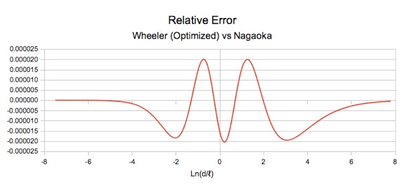
Note that the vertical scale has been magnified from that of the previous graphs.

The optimized version of Wheeler's formula using the fractional power term is:

(34)

where L_S is in µH; d= coil diameter (cm); ℓ =coil length (cm); N=number of turns.

Adjusted for SI units, the formula becomes:

(35)

where L_S is in Henries; d and ℓ are in meters.

It may prove even more useful when rearranged as an empirical formula for Nagaoka's coefficient:

(36)

where u = d/ℓ (dimensionless)

As mentioned earlier, the analytically derived coefficient 1.7636 does not affect asymptotic behaviour, but when doing these runs, and allowing the optimizer to adjust this value, the original analytical value turned out to be so close to optimum, that there was nothing to be gained by changing it.

Now, allow me to put on my engineer hat.

It's worth having another look at the analytically derived coefficients. In this analysis, while only shown to 4 or 5 decimal places, they were used at the maximum precision available in the software, which is about 15 significant figures. It's rather silly to offer this formula for general practical use with some coefficients deliberately optimized so that they may be truncated to 3 decimal places, and then require the other two constants to be applied at 15 digits of precision. As it happens, the analytically derived coefficients can be rounded to 5 decimal places with virtually no loss of accuracy. However, if these coefficients are to be truncated, it makes sense to do this before optimizing the empirical coefficients, in order that the optimization can offset whatever loss of accuracy occurs due to the truncation. With that in mind, I rounded the two analytically derived coefficients to 5 decimal places, and reran the optimization. The change in accuracy was too small to bother mentioning. However, since it did not decrease significantly, it seemed to be a worthwhile experiment to truncate the coefficients to 3 decimal places. The results were interesting. This optimization run produced the following values:

The maximum error in this case is 18.5 ppM. Ironically, by reducing precision, the accuracy is improved. These coefficients are incorporated in formula (37) as follows:

(37)

Although the increase in accuracy is hardly significant, this formula has some appeal, because k4 and e4 come out to be simple fractions. However, because of the truncation of k1, the formula is no longer asymptotic, and for that reason, it should not be used as the basis for a Nagaoka's coefficient function.

It remains a personal judgement call, whether the improved accuracy of these last formulae is worth the increased complexity. For comparison, Lundin's empirical formula [10] is accurate to 3 ppM, but is quite a bit more complicated, and in fact, consists of two separate formulae, one for short coils and one for long coils. However, any of the formulae presented on this page should be sufficiently accurate for most practical applications.

Running the Solver

You can run the solver and see how it converges on the optimum parameters. Select any or all of the input parameter cells, and then click the Solver button. For the target value cell, enter F20 or B12. The starting increment size of 0.1 can be used as in the previous example. For the Termination Std. Deviation, the value should be 1.0E-70, or else the calculation will tend to terminate too soon. Now, be warned that to optimize this function, the solver may need to run for a long time, depending on the starting values, and the number of variables the solver is optimizing. You don't have to wait for the solver to terminate by itself. If it appears to be making no progress, you can stop it by clicking the Cancel button. Doing it in stages, a couple of variables at a time, is often the most efficient approach.

I could go into tremendous detail on how to use the solver, but it's best simply to try it out, and see for yourself, the effect of changing various parameters.

Conclusion

The purpose of this section has been threefold; firstly, to present Wheeler's 1982 continuous inductance formula, and to encourage its use as a simple more accurate replacement for his earlier long coil formula; secondly to demonstrate how a solver routine can optimize such formula; and thirdly, as an introduction to doubly asymptotic empirical formulae. There are a great number of functions which are doubly asymptotic, and may good candidates for development of simpler empirical functions using computer optimization techniques.

Acknowledgement

My sincere thanks to David Knight for his valuable input during the writing of this page.

Continue to:

Part 4 – Geometric Mean Distance